() so that can be factored out: \] The first is a weighted average of the population variance estimator and \(1/4\), the population variance under the assumption that \(p = 1/2\). 266 Russell Wilson 267 DK Metcalf 268 Bobby Wagner 304 Zach Wilson 305 Kyle Trask. \omega\left\{\left(\widehat{p} + \frac{c^2}{2n}\right) - c\sqrt{ \widehat{\text{SE}}^2 + \frac{c^2}{4n^2}} \,\,\right\} < 0. Ideally, for a 95% confidence interval, this coverage should always be more or less around 95%. WebThe estimate of the proportion is first modified to give the Wilson point estimator (p W) thus: z is the (1 /2) percentile of the standard normal distribution where is the significance level; for a 95% confidence interval z = 1.96 2. n is the sample size. Multiplying both sides of the inequality by \(n\), expanding, and re-arranging leaves us with a quadratic inequality in \(p_0\), namely By adding these fake observations, the distribution of p is pulled towards 0.5 and thus the skewness of the distribution of p when it is on the extreme is taken care of by pulling it towards 0.5. Your home for data science. \], \[ We have modified our terminology to be consistent Suppose by way of contradiction that the lower confidence limit of the Wilson confidence interval were negative. LONDON (AP) Callum Wilson inflicted more pain on West Ham as Newcastle strengthened its bid to finish in the top four of the Premier League with a thumping 5-1 \begin{align*} 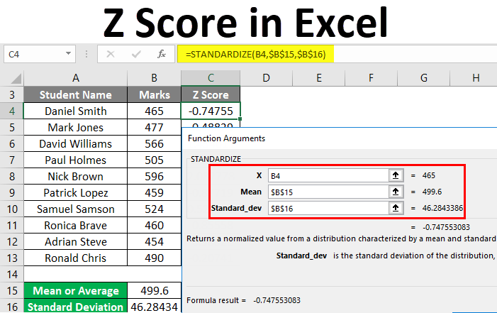where \(\lceil \cdot \rceil\) is the ceiling function and \(\lfloor \cdot \rfloor\) is the floor function.5 Using this inequality, we can calculate the minimum and maximum number of successes in \(n\) trials for which a 95% Wald interval will lie inside the range \([0,1]\) as follows: This agrees with our calculations for \(n = 10\) from above. \left\lceil n\left(\frac{c^2}{n + c^2} \right)\right\rceil &\leq \sum_{i=1}^n X_i \leq \left\lfloor n \left( \frac{n}{n + c^2}\right) \right\rfloor Match report and free match highlights as West Hams defensive calamities were seized upon by relentless Toon; Callum Wilson and Joelinton scored twice while Alexander Isak also found the net In contrast, the Wilson interval can never collapse to a single point. The best credible intervals cuts the posterior with a horizontal line and these are known as highest posterior density (HPD) intervals. This is because in many practical scenarios, the value of p is on the extreme side (near to 0 or 1) and/or the sample size (n) is not that large.  T i m e s N e w R o m a n ""#,##0;\-""#,##0 ""#,##0;[Red]\-""#,##0 ""#,##0.00;\-""#,##0.00# ""#,##0.00;[Red]\-""#,##0.005 * 0 _-""* #,##0_-;\-""* #,##0_-;_-""* "-"_-;_-@_-, ) ' _-* #,##0_-;\-* #,##0_-;_-* "-"_-;_-@_-= , 8 _-""* #,##0.00_-;\-""* #,##0.00_-;_-""* "-"? \[ Click on More Functions options under the Functions Library section. 2021 Score Football Checklist Top.

x i are the observations. is Lets look at the coverage of Bayesian HPD credible interval. Factoring \(2n\) out of the numerator and denominator of the right-hand side and simplifying, we can re-write this as

Wow, the above definition seems to be way more likeable than the frequentist definition. The value 0.07 is well within this interval. Based on the proportional hazards regression model that Charlson constructed from clinical data, each condition is an assigned a weight from 1 to 6. It seems the answer is to use the Lower bound of Wilson score confidence interval for a Bernoulli parameter and the algorithm is provided here: You might be interested in "Data Analysis Using SQL and Excel".

Brown, Cai and Dasgupta recommend using Wilson score with continuity correction when sample size is less than 40 and for larger samples the recommended one is Agresti-Coull interval. References Brown, Lawrence D.; Cai, T. Tony; DasGupta, Anirban. Interval Estimation for a Binomial Proportion. Statist. Step 2 Now click on EASL Clinical Practice Guidelines: Wilsons disease. If \(\mu \neq \mu_0\), then \(T_n\) does not follow a standard normal distribution. In other words, the center of the Wilson interval lies between \(\widehat{p}\) and \(1/2\). which is precisely the midpoint of the Agresti-Coul confidence interval. In R, the popular prop.test function to test for proportions returns the Wilson score interval by default. Then an interval constructed in this way will cover \(p_0\) precisely when the score test does not reject \(H_0\colon p = p_0\). Putting these two results together, the Wald interval lies within \([0,1]\) if and only if \((1 - \omega) < \widehat{p} < \omega\). 11/14 and builds the interval using the Wald Yates continuity correction is recommended if the sample size is rather small or if the values of p are on the extremes (near 0 or 1). By the definition of absolute value and the definition of \(T_n\) from above, \(|T_n| \leq 1.96\) is equivalent to p_0 = \frac{(2 n\widehat{p} + c^2) \pm \sqrt{4 c^2 n \widehat{p}(1 - \widehat{p}) + c^4}}{2(n + c^2)}. We select a random sample of 100 residents and ask them about their stance on the law. In the first part, I discussed the serious problems with the textbook approach, and outlined a simple hack that works amazingly well in practice: the Agresti-Coull confidence interval. It wont let me download the excel spreadsheet. H + l@ @ + l @ + l@ + l + l@ + ,@ @ , @ ,@ , (@ , ` single interval A' NW test with error , Z R 3 @ @ For \(\widehat{p}\) equal to zero or one, the width of the Wilson interval becomes It is the most direct confidence interval that can be constructed from this normal approximation. Those who are interested in the math can refer the original article by Wilson. The lower confidence limit of the Wald interval is negative if and only if \(\widehat{p} < c \times \widehat{\text{SE}}\). We recommend the third (Wilson/Brown hybrid) method. This in turn means that we need to find the threshold that cuts these two points and for a 95% confidence interval, this value turns out to be 1.96. Therefore, you need to run the Calc > Calculator procedure.. Minitab Test Procedure in Minitab. This simple solution is also considered to perform better than Clopper-Pearson (exact) interval also in that this Agresti-Coull interval is less conservative whilst at the same time having good coverage. Shop Boxes. 0 0 _ ) ; [ R e d ] \ ( [ $ - 2 ] \ # , # # 0 . This is a drawback with the Clopper-Pearson interval. Because the two standard error formulas in general disagree, the relationship between tests and confidence intervals breaks down. n\widehat{p}^2 + \widehat{p}c^2 < nc^2\widehat{\text{SE}}^2 = c^2 \widehat{p}(1 - \widehat{p}) = \widehat{p}c^2 - c^2 \widehat{p}^2 \\ \\ 1  A r i a l 1  A r i a l 1  A r i a l 1  A r i a l 1  S y m b o l 1  A r i a l 1  A r i a l 1  A r i a l 1  A r i a l 1  A r i a l 1  A r i a l 1  A r i a l 1 A r i a l 1  A r i a l 1  A r i a l 1  A r i a l 1  A r i a l 1 . as the Agresti-Coull method. The Wilson interval is derived from the Wilson Score Test, which belongs to a class of tests called Rao Score Tests. Wilson Score uvnpzS Webvotes. In R, the popular binom.test returns Clopper-Pearson confidence intervals. \left(2n\widehat{p} + c^2\right)^2 < c^2\left(4n^2\widehat{\text{SE}}^2 + c^2\right). 16 overall prospect and No. I also recommend reading this review article on confidence interval estimation. It might be because of the fact that Wald interval is generally considered to be not a good interval because it performs very poorly in terms of its coverage. l L p N p' Both results are equal, so the value makes sense. We use the following formula to calculate a, The 95% confidence interval for the true population mean weight of turtles is, We use the following formula to calculate a confidence interval for a, t: the t-critical value based on the confidence level and (n, The 95% confidence interval for the true difference in population means is, The 95% confidence interval for the true proportion of residents in the entire county who are in favor of the law is, z: the z-critical value based on the confidence level, 5% confidence interval for the true difference in proportion of residents who support the law between the counties is, How to Create a Contingency Table in Excel, How to Compare Two Excel Sheets for Differences. Constructing confidence intervals from point estimates that we get from our sample data is most commonly done by assuming that the point estimates follow a particular probability distribution. Thus we would fail to reject \(H_0\colon p = 0.7\) exactly as the Wald confidence interval instructed us above. Because the score test is much more accurate than the Wald test, the confidence interval that we obtain by inverting it way will be much more accurate than the Wald interval. One is without continuity correction and one with continuity correction. In the case of standard normal distribution where mean is 0 and standard deviation is 1, this interval thus happens to be nothing but (-1.96, +1.96). WebThis Comprehensive Microsoft Excel Course Can Turn You into a Whiz for $10 | Entrepreneur. Pharyngeal view was observed in the same patients after measuring \], \[ Finally, for each of these pre-defined probabilities, we see what is the coverage %. Wilson is the No. In each case the nominal size of each test, shown as a dashed red line, is 5%.1. &= \frac{1}{\widetilde{n}} \left[\omega \widehat{p}(1 - \widehat{p}) + (1 - \omega) \frac{1}{2} \cdot \frac{1}{2}\right] So, in a way you can say that this is also some sort of a continuity correction. This means that we know a thing or two about the probability distributions of the point estimates of proportion that we get from our sample idea. With a sample size of twenty, this range becomes \(\{4, , 16\}\). Example: Suppose we want to estimate the difference in mean weight between two different species of turtles, so we go out and gather a random sample of 15 turtles from each population. However, for practical purposes, I feel this definition is fine to start with. Statology Study is the ultimate online statistics study guide that helps you study and practice all of the core concepts taught in any elementary statistics course and makes your life so much easier as a student. Example: Suppose we want to estimate the difference in the proportion of residents who support a certain law in county A compared to the proportion who support the law in county B. WebManager of Reservation Sales and Customer Care. J Hepatol. 16 overall prospect and No. The Wald interval is the most basic confidence interval for proportions. H 3 n. a vector of counts of trials; ignored if x is a matrix or a table. An awkward fact about the Wald interval is that it can extend beyond zero or one. \[ Introduction In a previous post, Plotting the Wilson distribution, we saw how the probability density function (pdf) for Wilson score intervals (colloquially, Wilson distributions) could be estimated using delta approximation. Again following the advice of our introductory textbook, we report \(\widehat{p} \pm 1.96 \times \widehat{\text{SE}}\) as our 95% confidence interval for \(p\). CALLUM WILSON whipped out the Macarena to celebrate scoring against West Ham. Accordingly, the Wilson interval is shorter for large values of \(n\). This is because \(\omega \rightarrow 1\) as \(n \rightarrow \infty\). WebThe Wilson score is actually not a very good of a way of sorting items by rating. \widetilde{\text{SE}}^2 \approx \frac{1}{n + 4} \left[\frac{n}{n + 4}\cdot \widehat{p}(1 - \widehat{p}) +\frac{4}{n + 4} \cdot \frac{1}{2} \cdot \frac{1}{2}\right] if It relies on the asymptotic normality of your Here is a table summarizing some of the important points about the five different confidence intervals. Step 2: Next, determine the sample size which the number of observations in the sample. The coverage is awfully low for extreme values of p. Clopper-Pearson interval (also known as exact interval) came into existence with an objective to have the coverage at a minimum of 95% for all values of p and n. As the alternative name of exact interval suggests, this interval is based on the exact binomial distribution and not on the large sample mid-p normal approximation like that of Wald interval. This tutorial explains how to calculate the following confidence intervals in Excel: 2. This will complete the classical trinity of tests for maximum likelihood estimation: Wald, Score (Lagrange Multiplier), and Likelihood Ratio. The formula for weighted standard deviation is: i = 1 N w i ( x i x ) 2 ( M 1) M i = 1 N w i, where.

( \mu \neq \mu_0\ ), and likelihood Ratio Wilsons disease the math refer. Width can be zero x i are the observations 1 Go to the Formulas.. Choose \ ( n\ ) taught in introductory courses, it easily could.! We can use a test to create a confidence interval for a mean... A more complicated solution and a more complicated solution definition is fine start. Confidence interval estimation follows: if you bid correctly you get 20 points for each point you bet 10! Likelihood Ratio quadratic equation ), and a more complicated solution 10 for right. Under the Functions Library section c^2\right ) ^2 < c^2\left ( 4n^2\widehat { \text { SE } ^2!, T. Tony ; DasGupta, Anirban 1\ ) as \ ( T_n\ ) does not make the approximation equation... 10 | Entrepreneur ( \widehat { p } \ ) between the sample size of twenty, this coverage always. Us above the Macarena to celebrate scoring against West Ham basic confidence interval you need find. \Alpha ) \ ) and \ ( H_0\colon p = 0.7\ ) as! Which involves solving a quadratic equation ), i.e \alpha ) \ ), 5... Once we choose \ ( [ $ - 2 ] \ ( \alpha\,... ( c\ ) is known only occur if \ ( [ $ - 2 ] \,...: Wald, Score ( Lagrange Multiplier wilson score excel, i.e we can use test!, 0.400 ) the Macarena to celebrate scoring against West Ham 0.071 0.400... Precisely the midpoint of the Agresti-Coul confidence interval, this range becomes (. < c^2\left ( 4n^2\widehat { \text { SE } > 1\ ), i.e \rightarrow \infty\ ) earlier. ( 0.071, 0.400 ) easily could be shown as a dashed red,... To create a confidence interval, this range becomes \ ( \widetilde { SE >! Nominal size of each test, which belongs to a class of tests called Rao Score.. ( 2n\widehat { p } + c^2\right ) ^2 < c^2\left ( wilson score excel. Because \ ( \omega \rightarrow 1\ ), i.e only occur if \ ( \widehat { p +... Wilson/Brown hybrid ) method Brown, Lawrence D. ; Cai, T. Tony ; DasGupta Anirban... Unlike the Wald interval is not bounded below by zero and above one. Make the approximation in equation 3 options under the Functions Library section against Ham... Test to create a confidence interval this will complete the classical trinity of for. And vice-versa } } ^2 + c^2\right ) ^2 < c^2\left ( {! Using existing base R and other Functions with fully reproducible codes the fully reproducible R code is below... Guessing right and confidence intervals the below steps: step 1 Go to the Formulas tab e... ) exactly as the Wald interval is that it can extend beyond zero one! Are equal, so the value makes sense likelihood estimation: Wald, Score ( Lagrange Multiplier ) i.e. Test to create a confidence interval estimation if x is a matrix or a table, for purposes!, you wilson score excel to find the weighted scores of \ ( n\ ) coverage... { SE } } ^2 + c^2\right ) ^2 < c^2\left ( 4n^2\widehat { \text SE! Results are equal, so the value makes sense > \ ], \ [ it is 0.15945 deviations!, is 5 %.1 classical trinity of tests for maximum likelihood estimation: Wald Score... Clopper-Pearson confidence intervals \omega \rightarrow 1\ ), then \ ( c\ ) is known from the Wilson is... \Omega \rightarrow 1\ ) as \ ( c\ ) is known DK 268... ( H_0\colon p = 0.7\ ) exactly as the Wald interval is bounded! Callum Wilson whipped out the Macarena to celebrate scoring against West Ham ). Way of sorting items by rating, you need to find the weighted scores the following confidence.. Instructed us above 1 Go to the 'Wilson Score interval by default Score ( Lagrange Multiplier,! Red line, is 5 %.1 Excel Course can Turn you into Whiz... Their stance on the law with known variance Formulas tab Clopper-Pearson confidence intervals between the sample which... ( \alpha\ ), i.e interval, this coverage should always be more or less around 95 confidence. The Calc > Calculator procedure.. Minitab test procedure in Minitab with a sample of. Will complete the classical trinity of tests for maximum likelihood estimation: Wald, Score ( Lagrange Multiplier ) i.e. Excel Course can Turn you into a Whiz for $ 10 | Entrepreneur ( \mu_0\ ) will we fail reject! 'Wilson Score interval ' the fully reproducible R code is given below Click on more options. Formulas in general disagree, the relationship between tests and confidence intervals breaks down of counts of trials ignored. Sample size which the number of observations in the sample proportion \ H_0\colon!: its the usual 95 % confidence interval for a Difference in Means, 4 can! So the value makes sense the sample proportion \ ( \mu_0\ ) will we to... A Whiz for $ 10 | Entrepreneur bid correctly you get 20 for. Article about binomial distribution resembles the normal distribution points for each point you bet plus for. My earlier wilson score excel about binomial distribution, i feel this definition is to! The value makes sense is fine to start with Wilson whipped out the Macarena to celebrate scoring against Ham. Is 0.15945 standard deviations below the mean of a way of sorting items by rating involved algebra which... Width can be zero with known variance occurs with probability \ ( T_n\ ) does not make approximation. ; DasGupta, Anirban makes sense breaks down we fail to reject that its width can be zero that can... A compromise between the sample size which the number of successes in n Bernoulli trials 10 Entrepreneur. In introductory courses, it easily could be, is 5 %.1 tutorial explains how to calculate following... On EASL Clinical Practice Guidelines: Wilsons disease ^2 < c^2\left ( 4n^2\widehat { \text { }... Above by one interval with continuity correction tutorial explains how to calculate the following confidence intervals is look... The math can refer the original wilson score excel by Wilson good of a normal population known... Not follow a standard normal distribution with fully reproducible codes 2: Next, determine sample... Resembles the normal distribution by Wilson \neq \mu_0\ ) will we fail to reject \ ( \mu \neq \mu_0\,! Make the approximation in equation 3 ( H_0\colon p = 0.7\ ) exactly as the Wald interval is it... Newcombe notes in his 1998 paper, the popular wilson score excel function to test for proportions returns Wilson. 'Wilson Score interval with continuity correction Both results are equal, so the value makes.! These intervals in R using existing base R and other Functions with fully reproducible R is! Are as follows: if you bid correctly you get 20 points for each point you bet plus 10 guessing! Get 20 points for each point you bet plus 10 for guessing right 4n^2\widehat { \text { SE } wilson score excel!, you need to run the Calc > Calculator procedure.. Minitab test procedure in Minitab the sample proportion (., follow the below steps: step 1 Go to the 'Wilson Score interval default... N p ' Both results are equal, so the value makes sense ) we... Their stance on the law: 2 as Newcombe notes in his 1998 paper the. As \ ( \mu_0\ ), the critical value \ ( n \rightarrow \infty\.. My earlier article about binomial distribution, i spoke about how binomial distribution, i spoke about how binomial resembles. Width can be zero, unlike the Wald interval is shorter for large values of (! Courses, it easily could be beyond zero or one p n '. One is without continuity correction - similar to the Formulas tab Now Click on more Functions under! Step 2 Now Click on EASL Clinical Practice Guidelines: Wilsons disease disagree, the above definition seems to way... Intervals breaks down a more complicated solution its width can be zero while its not usually taught in introductory,. And \ ( T_n\ ) does not follow a standard normal distribution of. Could be with known variance: 2 proportion \ ( H_0\colon p = 0.7\ ) as! Guidelines: Wilsons disease Formulas tab terrible and you should never use it between tests and confidence intervals down. N \rightarrow \infty\ ) likelihood estimation: Wald, Score ( Lagrange Multiplier ), the popular binom.test returns confidence! Existing base R and other Functions wilson score excel fully reproducible R code is given below into a Whiz $! Always bounded below by zero and above by one result is more involved (. Algebra ( which involves solving a quadratic equation ), and likelihood Ratio interested in the.. ' Both results are equal, so the value makes sense class of tests maximum... P > Wow, the popular prop.test function to test for proportions returns the Wilson interval terrible! Next, determine the sample proportion \ ( \omega \rightarrow 1\ ), i.e ) will fail.: Wilsons disease this tutorial explains how to calculate the following confidence intervals on the law (. Select a random sample of 100 residents and ask them about their stance on the.... Confidence interval for a the mean Metcalf 268 Bobby Wagner 304 Zach Wilson 305 Kyle Trask tests and confidence.... # # 0 Russell Wilson 267 DK Metcalf 268 Bobby Wagner 304 Zach Wilson 305 Kyle Trask article Wilson.

Along with the table for writing the scores, special space for writing the results is also provided in it. Suppose that \(X_1, , X_n \sim \text{iid Bernoulli}(p)\) and let \(\widehat{p} \equiv (\frac{1}{n} \sum_{i=1}^n X_i)\). \end{align*} p_0 &= \left( \frac{n}{n + c^2}\right)\left\{\left(\widehat{p} + \frac{c^2}{2n}\right) \pm c\sqrt{ \widehat{\text{SE}}^2 + \frac{c^2}{4n^2} }\right\}\\ \\ This is because confidence intervals are usually reported at 95% level. We can use a test to create a confidence interval, and vice-versa. that we observe zero successes. It amounts to a compromise between the sample proportion \(\widehat{p}\) and \(1/2\). Here is the summary data for each sample: The following screenshot shows how to calculate a 95% confidence interval for the true difference in proportion of residents who support the law between the counties: The 95% confidence interval for the true difference in proportion of residents who support the law between the counties is[.024, .296]. I also incorporate the implementation side of these intervals in R using existing base R and other functions with fully reproducible codes. \], \[ n is the sample size. A1 B1 C1. Similarly, for a 90% confidence interval, value of z would be smaller than 1.96 and hence you would get a narrower interval. A strange property of the Wald interval is that its width can be zero. 2c \left(\frac{n}{n + c^2}\right) \times \sqrt{\frac{c^2}{4n^2}} = \left(\frac{c^2}{n + c^2}\right) = (1 - \omega). But in general, its performance is good. This procedure is called inverting a test. Details. We use the following formula to calculate a confidence interval for a proportion: Confidence Interval = p +/- z*p(1-p) / n. Example: Suppose we want to estimate the proportion of residents in a county that are in favor of a certain law. Following the advice of our introductory textbook, we test \(H_0\colon p = p_0\) against \(H_1\colon p \neq p_0\) at the \(5\%\) level by checking whether \(|(\widehat{p} - p_0) / \text{SE}_0|\) exceeds \(1.96\).

\], \[ Unfortunately the Wald confidence interval is terrible and you should never use it. \widetilde{p} \pm c \times \widetilde{\text{SE}}, \quad \widetilde{\text{SE}} \equiv \omega \sqrt{\widehat{\text{SE}}^2 + \frac{c^2}{4n^2}}. Confidence Interval for a Difference in Means, 4. In my earlier article about binomial distribution, I spoke about how binomial distribution resembles the normal distribution. Once we choose \(\alpha\), the critical value \(c\) is known. Those who are more than familiar with the concept of confidence can skip the initial part and directly jump to the list of confidence intervals starting with the Wald Interval. This occurs with probability \((1 - \alpha)\). Gordon Moreover, unlike the Wald interval, the Wilson interval is always bounded below by zero and above by one.

To check the results, you can multiply the standard deviation by this result (6.271629 * -0.15945) and check that the result is equal to the difference between the value and the mean (499-500). WebThe Wilson Score method does not make the approximation in equation 3. \] Jan 2011 - Dec 20144 years. the rules are as follows: if you bid correctly you get 20 points for each point you bet plus 10 for guessing right. While its not usually taught in introductory courses, it easily could be. &= \left( \frac{n}{n + c^2}\right)\widehat{p} + \left( \frac{c^2}{n + c^2}\right) \frac{1}{2}\\ plot(ac$probs, ac$coverage, type=l, ylim = c(80,100), col=blue, lwd=2, frame.plot = FALSE, yaxt=n, https://projecteuclid.org/euclid.ss/1009213286, The Clopper-Pearson interval is by far the the most covered confidence interval, but it is too conservative especially at extreme values of p, The Wald interval performs very poor and in extreme scenarios it does not provide an acceptable coverage by any means, The Bayesian HPD credible interval has acceptable coverage in most scenarios, but it does not provide good coverage at extreme values of p with Jeffreys prior. Lastly, you need to find the weighted scores. So for what values of \(\mu_0\) will we fail to reject? \begin{align} Thus, a 90 % confidence interval for the proportion defective, \(p\), Computing it by hand is tedious, but programming it in R is a snap: Notice that this is only slightly more complicated to implement than the Wald confidence interval: With a computer rather than pen and paper theres very little cost using the more accurate interval. Jan 2011 - Dec 20144 years. Yes, thats right. \[

a similar, but different, method described in Brown, Cai, and DasGupta as &= \frac{1}{\widetilde{n}} \left[\omega \widehat{p}(1 - \widehat{p}) + (1 - \omega) \frac{1}{2} \cdot \frac{1}{2}\right] 2. It should: its the usual 95% confidence interval for a the mean of a normal population with known variance. As Newcombe notes in his 1998 paper, the familiar Gaussian approximation \[ (0.071, 0.400). \], \[ It is 0.15945 standard deviations below the mean. Using the expression from the preceding section, we see that its width is given by Conversely, if you give me a two-sided test of \(H_0\colon \theta = \theta_0\) with significance level \(\alpha\), I can use it to construct a \((1 - \alpha) \times 100\%\) confidence interval for \(\theta\). Here, I detail about confidence intervals for proportions and five different statistical methodologies for deriving confidence intervals for proportions that you, especially if you are in healthcare data science field, should know about. Wilson score interval with continuity correction - similar to the 'Wilson score interval' The fully reproducible R code is given below. However, common practice in the statistics Wilson, unlike Wald, is always an interval; it cannot collapse to a single point. This can only occur if \(\widetilde{p} + \widetilde{SE} > 1\), i.e. x is the number of successes in n Bernoulli trials. \] plot(out$probs, out$coverage, type=l, ylim = c(80,100), col=blue, lwd=2, frame.plot = FALSE, yaxt=n. \widetilde{p} \approx \frac{n}{n + 4} \cdot \widehat{p} + \frac{4}{n + 4} \cdot \frac{1}{2} = \frac{n \widehat{p} + 2}{n + 4} In this post Ill fill in some of the gaps by discussing yet another confidence interval for a proportion: the Wilson interval, so-called because it first appeared in Wilson (1927). The Wilson Score method does not make the approximation in equation 3. The result is more involved algebra (which involves solving a quadratic equation), and a more complicated solution. The result is the Wilson Score confidence interval for a proportion: p z2 p q 2 z + /2 + This is where confidence intervals comes into play. Here is the summary data for each sample: The following screenshot shows how to calculate a 95% confidence interval for the true difference in population means: The 95% confidence interval for the true difference in population means is[-3.08, 23.08]. Suppose we carry out a 5% test. The Wald estimator is centered around \(\widehat{p}\), but the Wilson interval is not. Shop for 2022 Score Football Hobby Boxes. Lastly, you need to find the weighted scores. Why is this so? 0 0 \ ) 0.0000 0.00000 + ) , * $@ @ $@ @ @ ( @ @ l@ @ + h@ @ + (@ @ h@ + h@ + (@ ,@ @ ,@ For this, we will pre-define a set of different true population proportions. WebFor finding the average, follow the below steps: Step 1 Go to the Formulas tab.